详解MegatronLM序列模型并行训练(Sequence Parallel)
1. 背景介绍
MegatronLM的第三篇论文【Reducing Activation
Recomputation in Large Transformer
Models】是2022年出的。在大模型训练过程中显存占用过大往往成为瓶颈,一般会通过recomputation重计算的方式降低显存占用,但会带来额外的计算代价。这篇论文提出了两种方法,分别是sequece parallel和selective activation recomputation,这两种方法和Tensor并行是可以相结合的,可以有效减少不必要的计算量。
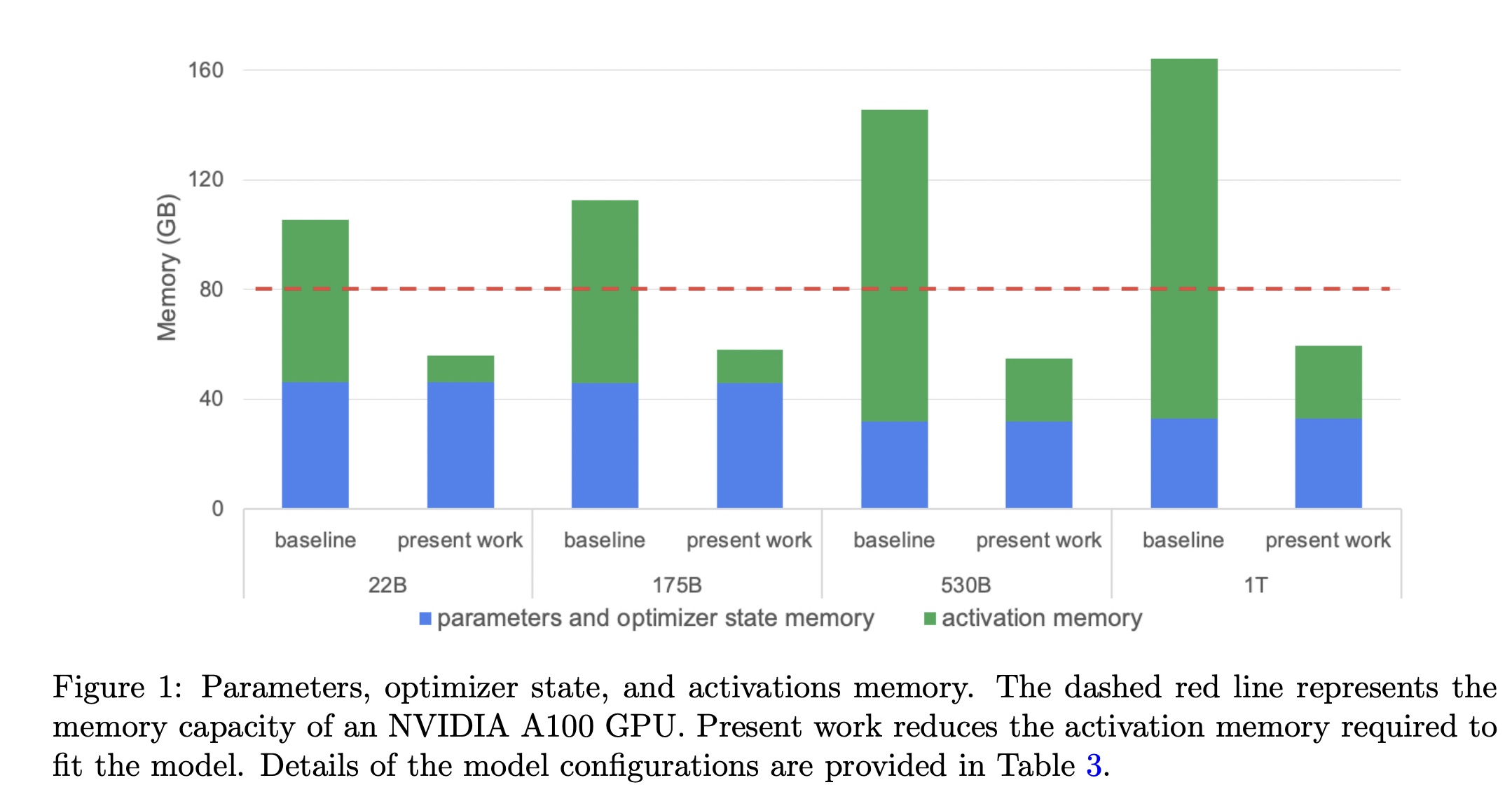
下图中绿色部分表示不同模型中需要用于保存activation需要的显存大小,蓝色部分表示不同模型中需要用于保存parameter和optimizer state需要的显存大小。红色线表示A100的显存大小80G。
2. Pipeline Parallel详细介绍
2.1 估算Transformer Activation Memory大小
以Transformer结构为例估算Activation Memory大小,这里的Activation定义是指前向和反向梯度计算中创建的所有tensor。按这个定义来说,计算不包含模型参数大小和优化器中状态大小,但是包含dropout
op用到的mask tensor。
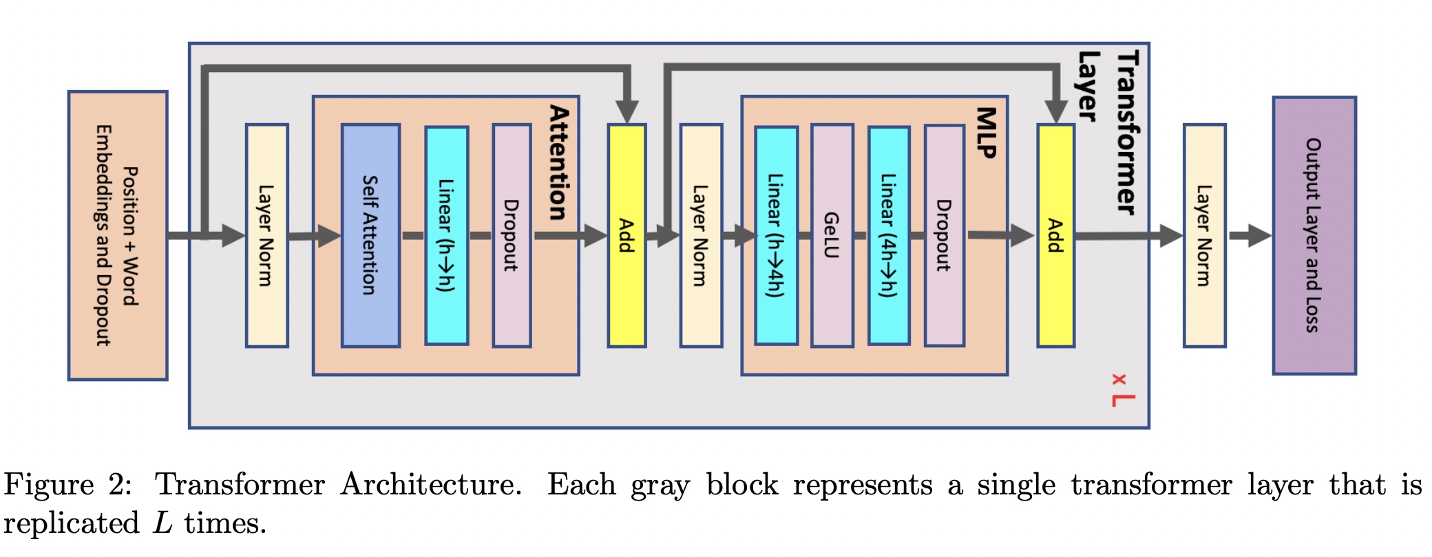
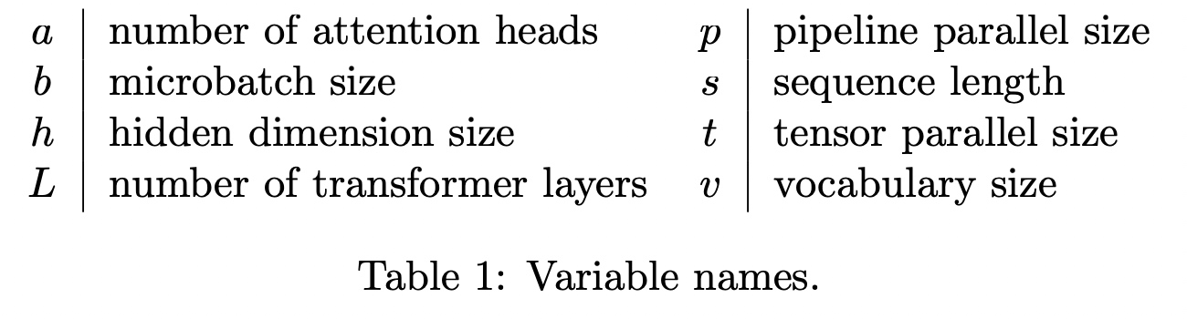
一个Transformer块中由一个Attention块和一个MLP块组成,中间通过两个LayerNorm层进行连接。在Transformer中用到的参数表示如下:
Attention模块的计算公式如下:
\[\begin{gather*} Attention(Q, K, V) = softmax(\frac{QK^T}{\sqrt{d_k}})V \end{gather*}\]
对于Attention块来说,输入的element个数为sbh个,每个element以16-bit的浮点数(也就是2
bytes)来进行存储的话,对应输入的element大小为2sbh bytes,后续计算默认都是按bytes为单位进行计算。
Attention块中包含一个self-attention块、一个linear线性映射层和attention dropout层。对于linear线性映射层来说需要保存输入的Activation大小为2sbh,
对于attention dropout层需要mask的大小为sbh(对于一个元素的mask只用1个bytes即可),对于self-attention块的Activation Memory的计算有以下几块:
* \(Query(Q), Key(K), Value
(V)\)矩阵相乘:输入input是共享的,元素个数为sbh个,总大小是
2sbh bytes。 * \(QK^T\)
矩阵相乘:需要分别创建保存 \(Q\) 和
\(K\) 的矩阵,每个矩阵元素总大小为
2sbh bytes, 总共大小为 4sbh
bytes。如下图以b=1, s=2, h=6为例,输入\(X\)元素个数为1 * s * h = 12个,计算完后\(Q\) 和 \(K\) 的矩阵中元素个数各有
1 * s * h = 12个,总元素大小为2 * 2 * b * s * h = 48
bytes。 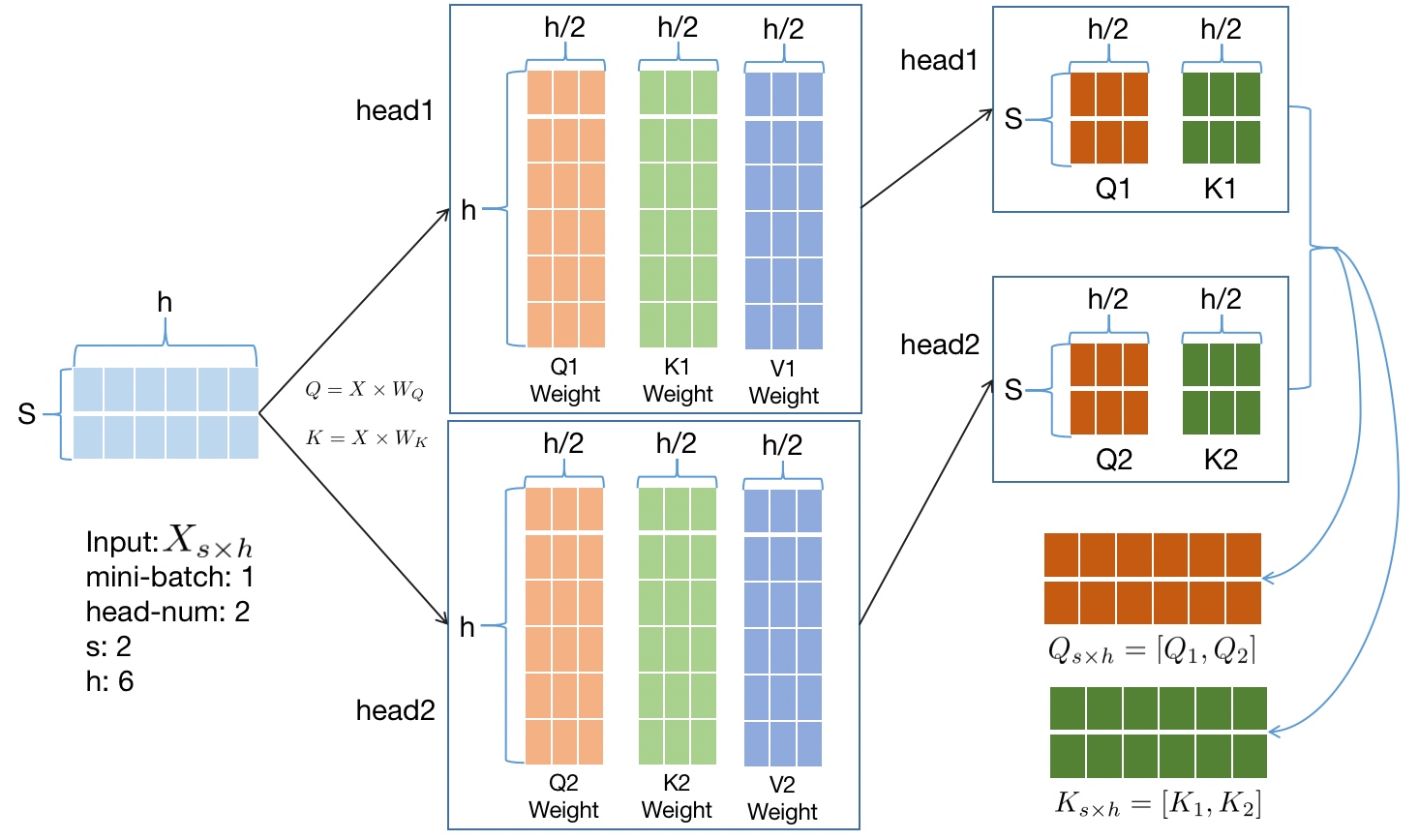
- softmax的输出总的元素大小为\(2as^2b\) bytes, 分别计算每个Head头的\(Q_n \times K_n\) 的乘积。计算公式如下,
图中计算以
b=1, s=2, h=6, a=2为例:
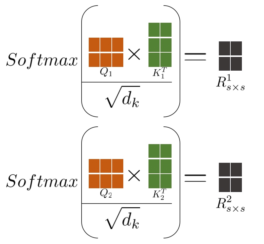
- 在softmax后还有dropout的mask层大小,mask矩阵的大小与softmax的输出一样,元素个数都是 \(as^2b\) 个,但mask单个元素的大小只用1 bytes即可,总的大小为 \(as^2b\) bytes
- softmax的输出也会用于反向的计算,需要缓存下来,对应大小也是 \(2as^2b\)
- \(V\) 矩阵的大小之前没有统计,和
\(Q\)、\(K\)矩阵一样,大小也是
2sbhbytes
综上,Attention Block总的大小为 11sbh + 5as^2b
bytes。
MLP的Activation大小计算:MLP中有两层线性layer,分别存储输入矩阵大小为
\(2sbh\) bytes和 \(8sbh\)
bytes;GeLU的反向也需要对输入进行缓存,大小为 \(8sbh\) bytes; dropout层需要
sbh bytes; 总大小为 19sbh。
LayerNorm的Activation大小计算:每个LayerNorm层的输入需要 \(2sbh\) 大小,有两个LayerNorm层,总大小为
4sbh bytes.
最终transformer网络中一层(含Attention/MLP/LayerNorm)的Activation总的大小为:
\[\begin{gather} ActivationMemoryPerLayer = sbh \left( 34 + 5 \frac{as}{h} \right) \end{gather}\]
注意: 这里公式(1)计算的Activation总和是在没有应用模型并行策略的前提下进行的。
2.2 Tensor Parallel的Activation Memory计算
如下图,在Tensor模型并行中只在Attention和MLP两个地方进行了并行计算,对于Attention(Q/K/V)和MLP(Linear Layer)的输入并没有并行操作。图中 \(f\) 和 \(\overline{f}\) 互为共轭(conjugate),\(f\) 在前向时不做操作,反向时执行all-reduce; \(\overline{f}\) 在前向时执行all-reduce, 反向时不做操作。

参虑上Tensor并行的话(Tensor并行度为 \(t\)),并行部分有MLP的Linear部分(\(18sbh\) bytes)和Attention的QKV部分(\(6sbh\) bytes),
ActivationMemoryPerLayer相比公式(1)中的值降为: \[\begin{gather}
ActivationMemoryPerLayer = sbh \left( 10 + \frac{24}{t} + 5 \frac{as}{h}
\right)
\end{gather}\]
2.2 Sequence Parallel
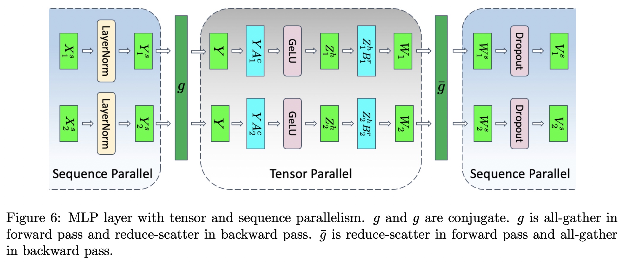
在Tensor模型并行基础上提出了Sequence Parallel,对于非Tensor模型并行的部分在sequence维度都是相互独立的,所以可以在sequence维度上进行拆分(即sequence parallel)。拆分后如下图,\(f\) 和 \(\overline{f}\) 替换为 \(g\) 和 \(\overline{g}\), \(g\) 和 \(\overline{g}\) 也是共轭的,\(g\)
在前向是all-gather通信,反向是reduce-scatter通信;\(\overline{g}\)在前向是reduce-scatter,
反向是all-gather通信。
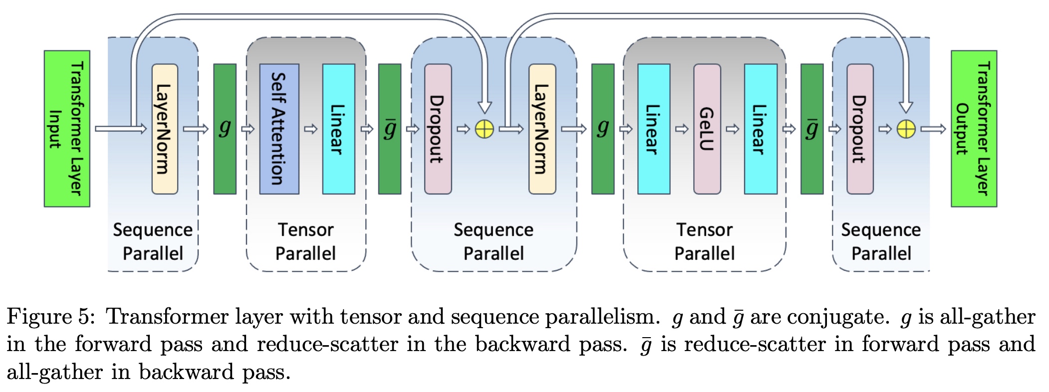
接下来以MLP为例,详细说明拆分步骤。MLP层由两个Linear层组成,对应的计算公式如下, 其中 \(X\) 的大小为 \(s \times b \times h\) ; \(A\) 和 \(B\) 是Linear的权重weight矩阵,大小为 \(h \times 4h\) 和 \(4h \times h\)。
\[\begin{gather*} \begin{aligned} Y &= LayerNorm(X) \\ Z &= GeLU(YA) \\ W &= ZB \\ V &= Dropout(W) \\ \end{aligned} \end{gather*}\]
如下图,切分时说明如下: 1. 对 \(X\) 按sequence维度切分,\(X = \left[ X^s_1, X^s_2 \right]\),LayerNorm的结果 \(Y = \left[ Y^s_1, Y^s_2 \right]\); 2. 由于接下来的GeLU不是线性的,所以要进行all-gather操作,计算 \(Z = GeLU(YA)\); 3. 对 \(A\) 进行列切分的tensor并行,得到结果 \(YA^c_1\) 和 \(YA^c_2\) 4. 对 \(B\) 进行行切分的tensor并行,得到结果 \(Z^h_1 B^r_1\) 和 \(Z^h_2 B^r_2\) 5. 得到 \(W_1\) 和 \(W_2\) 后进行累加操作(reduce-scatter)
对应的计算公式如下:
\[\begin{gather} \begin{aligned} \left[ Y^s_1, Y^s_2 \right] &= LayerNorm([X^s_1, X^s_2]) \\ Y &= g(Y^s_1, Y^s_2) \\ \left[ Z^h_1, Z^h_2 \right] &= [GeLU(YA^c_1), GeLU(YA^c_2)] \\ W_1 &= Z^h_1 B^r_1 \\ W_2 &= Z^h_2 B^r_2 \\ \left[ W^s_1, W^s_2 \right] &= \overline{g}(W_1, W_2) \\ \left[ V^s_1, V^s_2 \right] &= [Dropout(W^s_1), Dropout(W^s_2)] \\ \end{aligned} \end{gather}\]
Tensor并行在一次前向和后向总共有4次的all-reduce操作,在Sequence并行一次前向和后向总共有4次all-gather和4次reduce-scatter操作。ring all-reduce
执行过程中有两步,先是一个reduce-scatter然后跟着一个all-gather,Sequence并行相比没有引入更多的通信代价。一个使用reduce-scatter和all-gather实现all-reduce的Python代码示例如下:
1 | import torch |
通过使用sequence parallel和tensor parallel以后,ActivationMemoryPerLayer相比公式(2)的值再次减少,相比公式(1)相当于对所有的ActivationMemory进行Tensor并行,
即 \(\frac{ActivationMemoryPerLayer}{t}\):
\[\begin{gather} \begin{aligned} ActivationMemoryPerLayer &= sbh \left( \frac{10}{t} + \frac{24}{t} + 5 \frac{as}{ht} \right) \\ &= \frac{sbh}{t} \left( 34 + 5 \frac{as}{h} \right) \\ \end{aligned} \end{gather}\]
2.3 Pipeline Parallel
加上Pipeline Parallel后,对具有 \(L\)
层的layer的transformer来说,Pipeline Parallel并行度为 \(p\), 对应会分为 \(\frac{L}{p}\)
组(即stage个数)。以PipeDream中的1F1B调度为例,要完成初始化的话,第1个stage必须处理完
\(p\)
个micro-batch,让其他stage至少有1个micro-batch在处理,也就是要缓存 \(p\)
个micro-batch的activation。由于每个stage都有 \(\frac{L}{p}\) 个Layer,一共需要 \(p \times \frac{L}{p} = L\)
个layer的activation信息,对应总的计算如下:
\[\begin{gather} TotalActivationMemory = \frac{sbhL}{t} \left( 34 + 5 \frac{as}{h} \right) \\ \end{gather}\]
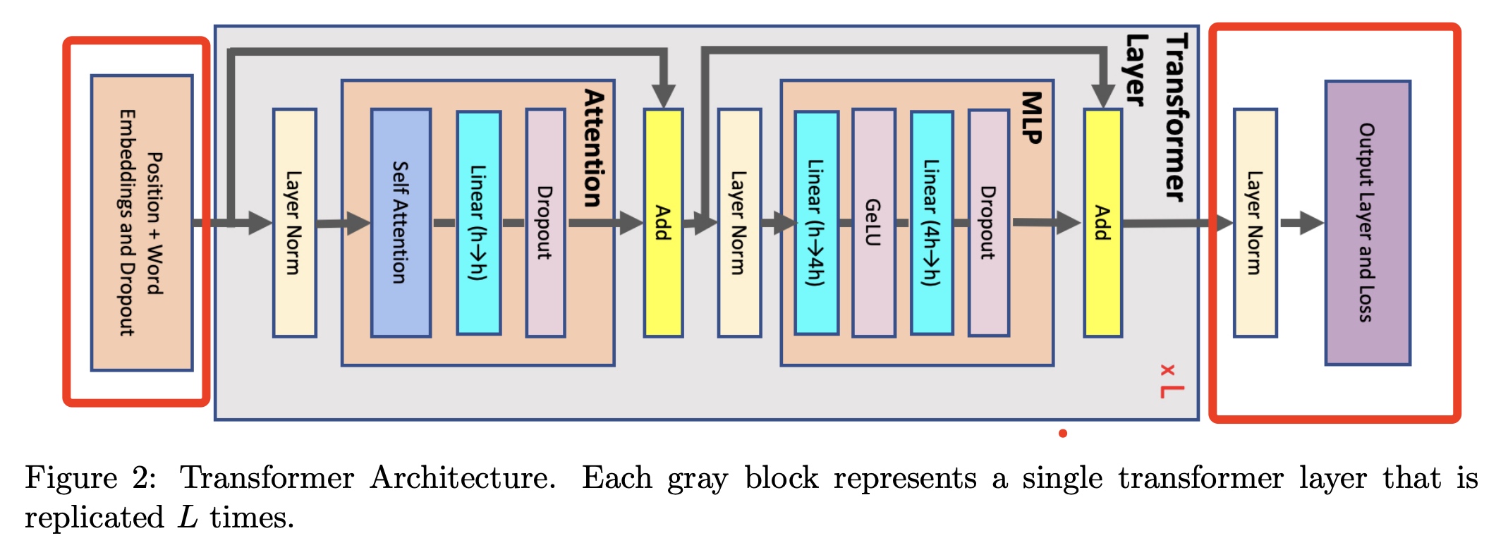
当然这里的公式(5)的ActivationMemory的计算没有加上EmbeddingLayer、最后的LayerNorm和输出的OutputLayer。加上这三部分的结果会略大于公式(5),
但以22B参数模型来说只增加0.01%的大小,这部分可忽略,证明请参考原论文。未计算部分如下图红色部分:
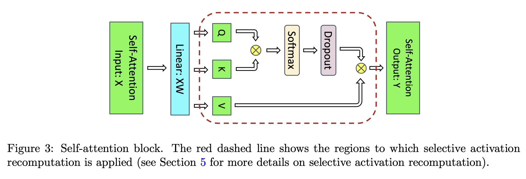
3. 可选Activation重计算介绍(Selective Activation Recomputation)
在后向过程中通过重计算方式重新计算前向结果来节省显存大小,这种方式文中称为full activation recomputation,以transformer为例会增加30%~40%的计算量。Selective的方式主要思路是选择
FLOPs 计算量小,且activation占用大的算子进行重计算,这里的
FLOPs
的衡量标准是GEMM的计算量大小。以公式(5)为例,针对大模型来说 \(5as/h \gt 34\),
如果重计算这部分layer的话可以减少快一半的activation大小。对于GPT-3来说,这种方式可以减少70%的activation显存大小,同时只增加了2.7%的
\(FLOPs\)
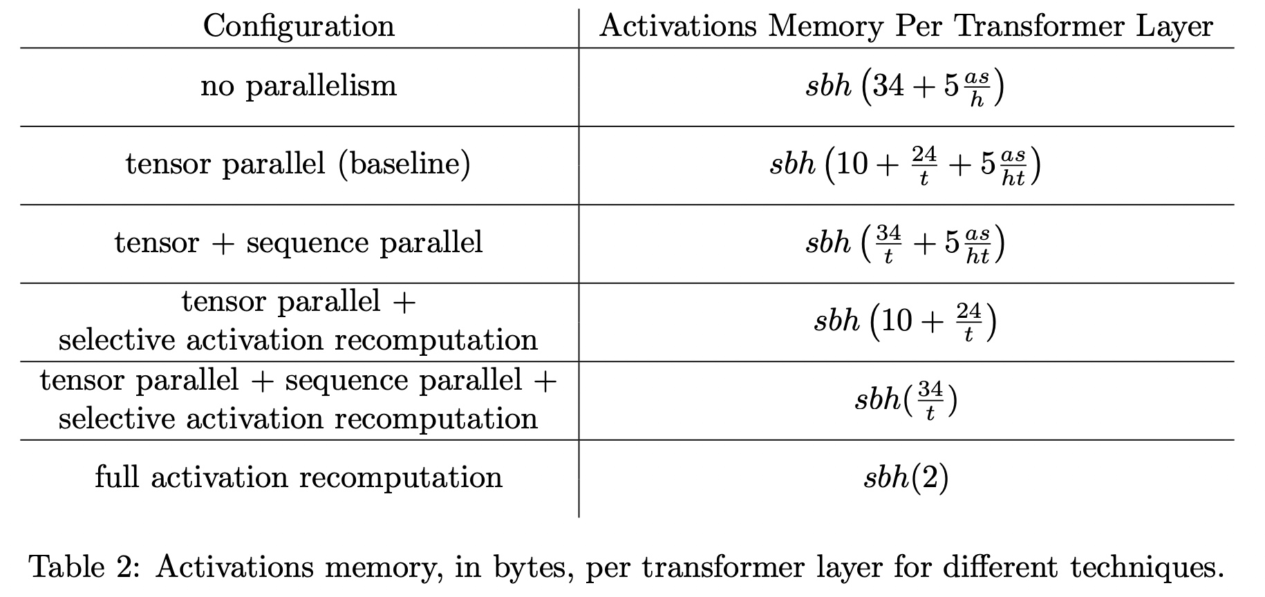
计算量。采用Selective Activation Recomputation后,公式(5)的结果可以减少为:
\[\begin{gather*} Total\ required\ memory = 34 \frac{sbhL}{t} \\ \end{gather*}\]
以下是不同方法组合下Activation Memory占用情况: